Loading Spectral Fitting Results
[ ]:
from astropy.io import fits
import numpy as np


scale_factor = 2
a = fits.open('mr2251.fits')[1].data.shape[1] // scale_factor
b = fits.open('mr2251.fits')[1].data.shape[2] // scale_factor

folder_names = [
    'reduced2',

    # 'reduced2_i83_93',

    # 'reduced2_i93_83',

    # 'reduced2_j90_100',

    # 'reduced2_j100_90',

    # 'reduced2_i76_66',

    # 'reduced2_i101_111',

    # 'reduced2_j81_71',

    # 'reduced2_j109_119',


    # 'reduced2_median',
    # 'reduced2_flat'

    # 'reduced2_selected'


]


# Create folder map, extract suffix after 'reduced2'. If not present, use an empty string
folder_map = {
    folder: f"_{folder[len('reduced2')+1:]}" if folder.startswith('reduced2_') else ''
    for folder in folder_names
}

print(folder_map)

# Initialize storage dictionary for dynamically created variables
data_arrays = {}
# Dynamically generate global variables
for suffix in folder_map.values():
    globals()[f'ha_flux{suffix}'] = np.full((a, b), np.nan)
    globals()[f'ha_vel{suffix}'] = np.full((a, b), np.nan)
    globals()[f'hb_vel{suffix}'] = np.full((a, b), np.nan)
    globals()[f'ha_sigma{suffix}'] = np.full((a, b), np.nan)
    globals()[f'O3_flux{suffix}'] = np.full((a, b), np.nan)
    globals()[f'O3_vel{suffix}'] = np.full((a, b), np.nan)
    globals()[f'O3_sigma{suffix}'] = np.full((a, b), np.nan)
    globals()[f'chi2{suffix}'] = np.full((a, b), np.nan)
    globals()[f'snr{suffix}'] = np.full((a, b), np.nan)
    globals()[f'habr1_flux{suffix}'] = np.full((a, b), np.nan)
    globals()[f'habr1_vel{suffix}'] = np.full((a, b), np.nan)
    globals()[f'habr1_sigma{suffix}'] = np.full((a, b), np.nan)
    globals()[f'habr2_flux{suffix}'] = np.full((a, b), np.nan)
    globals()[f'habr2_vel{suffix}'] = np.full((a, b), np.nan)
    globals()[f'habr2_sigma{suffix}'] = np.full((a, b), np.nan)

    globals()[f'ha_brflux{suffix}'] = np.full((a, b), np.nan)

# Iterate through each point and read data from corresponding folders
for folder, suffix in folder_map.items():
    for i in range(a):
        for j in range(b):
            try:
                # Open the FITS file in the corresponding folder
                spec = fits.open(f'./{folder}/{i}_{j}.fits')[1].data

                # Dynamically fill data from different regions into corresponding global variables

                globals()[f'ha_flux{suffix}'][i, j] = spec['Ha_na_1_scale'][0]
                globals()[f'ha_vel{suffix}'][i, j] = spec['Ha_na_1_centerwave'][0]
                globals()[f'hb_vel{suffix}'][i, j] = spec['Hb_na_1_centerwave'][0]
                globals()[f'ha_sigma{suffix}'][i, j] = spec['Ha_na_1_sigma'][0]
                # globals()[f'O3_flux{suffix}'][i, j] = spec['OIII4959c_1_scale'][0]
                # globals()[f'O3_vel{suffix}'][i, j] = spec['OIII4959c_1_centerwave'][0]
                # globals()[f'O3_sigma{suffix}'][i, j] = spec['OIII4959c_1_sigma'][0]
                globals()[f'chi2{suffix}'][i, j] = spec['2_line_red_chi2'][0]
                globals()[f'snr{suffix}'][i, j] = spec['Ha_whole_br_snr'][0]
                # globals()[f'habr1_flux{suffix}'][i, j] = spec['Ha_br1_1_scale'][0]
                # globals()[f'habr1_vel{suffix}'][i, j] = spec['Ha_br1_1_centerwave'][0]
                # globals()[f'habr1_sigma{suffix}'][i, j] = spec['Ha_br1_1_sigma'][0]
                # globals()[f'habr2_flux{suffix}'][i, j] = spec['Ha_br2_1_scale'][0]
                # globals()[f'habr2_vel{suffix}'][i, j] = spec['Ha_br2_1_centerwave'][0]
                # globals()[f'habr2_sigma{suffix}'][i, j] = spec['Ha_br2_1_sigma'][0]


                globals()[f'ha_brflux{suffix}'][i, j] = spec['Ha_whole_br_area'][0]

                print(f"current loop progress:folder = {folder}, i = {i}, j = {j}", end='\r')

            except:
                continue
[ ]:
%whos
Select the Best Fitting Results
[2]:
import matplotlib.pyplot as plt
imin = 0
imax = a
jmin = 0
jmax = b
import numpy as np
# Create a copy of the array to store the filtered results
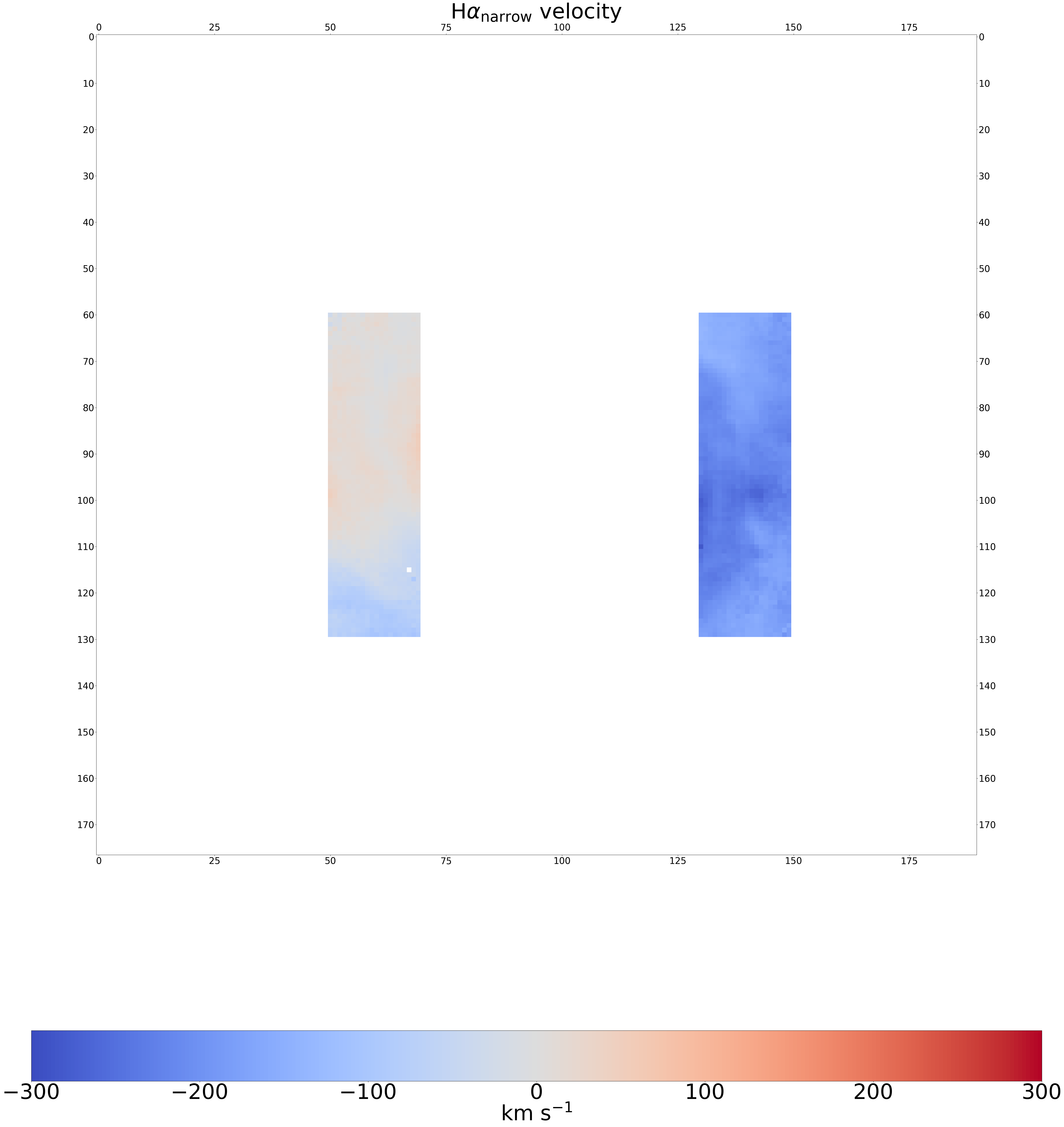
vel_filtered = ha_vel.copy()
sigma_filtered = ha_sigma.copy()
vel_filtered[0:,0:] = np.nan
sigma_filtered[0:,0:] = np.nan
# Manually keep two smooth and physical regions as initial reference
vel_filtered[60:130,50:70] = ha_vel.copy()[60:130,50:70]
sigma_filtered[60:130,50:70] = ha_sigma.copy()[60:130,50:70]
vel_filtered[60:130,130:150] = ha_vel.copy()[60:130,130:150]
sigma_filtered[60:130,130:150] = ha_sigma.copy()[60:130,130:150]
sigma = np.nanmean(sigma_filtered[imin:imax,jmin:jmax])
# Iterate over the array (excluding boundary points) and remove outliers
for _ in range(2):
for i in range(vel_filtered.shape[0]):
for j in range(vel_filtered.shape[1]):
if np.isnan(vel_filtered[i, j]):
continue # 跳过 NaN 的点
# Determine the neighboring region dynamically to avoid out-of-bounds
i_min = max(0, i - 1) # 行的最小索引
i_max = min(vel_filtered.shape[0], i + 2) # 行的最大索引
j_min = max(0, j - 1) # 列的最小索引
j_max = min(vel_filtered.shape[1], j + 2) # 列的最大索引
# Extract neighbors, excluding the current point
neighbors = vel_filtered[i_min:i_max, j_min:j_max].flatten() # 获取周围一圈的邻居
neighbors_sigma = sigma_filtered[i_min:i_max, j_min:j_max].flatten() # 获取周围一圈的邻居
neighbors = neighbors[neighbors != vel_filtered[i, j]] # 排除自身点
neighbors_sigma = neighbors_sigma[neighbors_sigma != sigma_filtered[i, j]] # 排除自身点
valid_neighbors = neighbors[~np.isnan(neighbors)] # 去除 NaN 值的邻居
valid_neighbors_sigma = neighbors_sigma[~np.isnan(neighbors_sigma)] # 去除 NaN 值的邻居
if len(valid_neighbors) > 2:
# Calculate the average difference between current value and neighbors
diffs = np.abs(vel_filtered[i, j] - np.array(valid_neighbors))
avg_diff = np.mean(diffs)
# If the current point is significantly higher or lower than all neighbors, and the difference > sigma
if (vel_filtered[i, j] > max(valid_neighbors) or vel_filtered[i, j] < min(valid_neighbors)) and avg_diff > sigma:
# Replace its sigma value with the median of its neighbors'
sigma_filtered[i, j] = np.median(valid_neighbors_sigma)
# And mark it as NaN (exclude this outlier)
vel_filtered[i, j] = np.nan
print("Filtered vel array:")
# Plot the filtered Hα narrow component velocity map
imin , imax, jmin, jmax = 0, a, 0, b
plt.figure(figsize=(60,70),dpi=100)
plt.imshow((np.e**(vel_filtered[imin:imax, jmin:jmax]) - 6564.4) / 6564.4 * 3e5 ,vmin = -300, vmax= 300, cmap='coolwarm' )
y_ticks = np.arange(0, (imax - imin) + 1, 10)
plt.yticks(y_ticks)
plt.tick_params(axis='both', which='major', labelsize=30)
plt.tick_params(axis='both', which='both', bottom=True, top=True, left=True, right=True, labelbottom=True, labeltop=True, labelleft=True, labelright=True)
plt.title(r'H$\alpha_{\rm narrow}$ velocity ',fontsize=70)
clb=plt.colorbar(orientation='horizontal')
clb.ax.tick_params(labelsize=70)
clb.ax.set_xlabel(r'km s$^{-1}$',fontsize=70)
过滤后的 vel 数组:
[2]:
Text(0.5, 0, 'km s$^{-1}$')
[5]:
from tqdm import tqdm
f1 = 1.5
f2 = 5
imin , imax, jmin, jmax = 0, a, 0, b
# Compute the average sigma from the filtered data
sigma0 = np.nanmean(sigma_filtered[imin:imax,jmin:jmax])
# Directly compute the lower and upper velocity bounds
lower_bound = (np.e**(vel_filtered[imin:imax, jmin:jmax] - 1 * sigma0) - 6564.4) / 6564.4 * 3e5
upper_bound = (np.e**(vel_filtered[imin:imax, jmin:jmax] + 1 * sigma0) - 6564.4) / 6564.4 * 3e5
# Estimate the typical velocity error
sigma = np.median((upper_bound - lower_bound)[~np.isnan(upper_bound - lower_bound)]) / 2
print('sigma:',sigma)
# Collect all candidate velocity, sigma, and chi2 maps
image_data_sources = [ha_vel, ha_vel_i83_93, ha_vel_i93_83, ha_vel_j90_100,
ha_vel_j100_90, ha_vel_i76_66, ha_vel_i101_111, ha_vel_j81_71, ha_vel_j109_119]
sigma_data_sources = [ha_sigma, ha_sigma_i83_93, ha_sigma_i93_83, ha_sigma_j90_100,
ha_sigma_j100_90, ha_sigma_i76_66, ha_sigma_i101_111, ha_sigma_j81_71, ha_sigma_j109_119]
chi2_data_sources = [chi2, chi2_i83_93, chi2_i93_83, chi2_j90_100,
chi2_j100_90, chi2_i76_66, chi2_i101_111, chi2_j81_71, chi2_j109_119]
# Precompute velocities for all candidate maps
image_velocity_list = [(np.e**data[imin:imax, jmin:jmax] - 6564.4) / 6564.4 * 3e5 for data in image_data_sources]
sigma_list = [data[imin:imax, jmin:jmax] for data in sigma_data_sources]
chi2_list = [data[imin:imax, jmin:jmax] for data in chi2_data_sources]
# Initialize with the first image
image_selected = image_velocity_list[0].copy()
sigma_selected = sigma_list[0].copy()
chi2_selected = chi2_list[0].copy()
# Identify outliers in the first image
# Define Select Region
normal_mask = (image_selected > lower_bound) & (image_selected < upper_bound) & (sigma_selected <= f2 * sigma0)&(chi2_selected<1000)
outliers_mask = ~normal_mask # Mask outliers as NaN
image_selected[outliers_mask] = np.nan
# Define function to compute local gradient
def gradient_sum(image, i, j):
"""
Calculate the sum of absolute differences in the 8-neighborhood around (i, j)
"""
grad_sum = 0
directions = [(-1, 0), (1, 0), (0, -1), (0, 1), (-1, -1), (-1, 1), (1, -1), (1, 1)]
for di, dj in directions:
ni, nj = i + di, j + dj
if 0 <= ni < image.shape[0] and 0 <= nj < image.shape[1] and not np.isnan(image[ni, nj]):
grad_sum += abs(image[ni, nj] - image[i, j])
return grad_sum
# Select Valid Results
for idx, image in enumerate(image_velocity_list[1:], 1):
for i in range(image_selected.shape[0]):
for j in range(image_selected.shape[1]):
conditions_met = (
lower_bound[i, j] <= image[i, j] <= upper_bound[i, j] and
sigma_list[idx][i, j] <= f2 * sigma0 and
chi2_list[idx][i, j] < 1000
)
# If the first image has NaN at this point, try to find a valid value from other images
if np.isnan(image_selected[i, j]):
if conditions_met: # A valid value is found
image_selected[i, j] = image[i, j] # Assign the value and stop searching
# If the first image is not NaN at this point, check the other images
else:
if conditions_met:
# If the current image is valid, calculate gradient smoothness
current_grad = gradient_sum(image_selected, i, j)
temp_image = image_selected.copy()
temp_image[i, j] = image[i, j]
new_grad = gradient_sum(temp_image, i, j)
if new_grad < current_grad:
# Replace the value if the new one leads to smoother gradient
image_selected[i, j] = image[i, j]
# Fill Missing Point
def fill_nan_with_median(image):
"""
Fill NaN points in the image using the median of surrounding non-NaN neighbors.
"""
filled_image = np.copy(image)
for i in range(image.shape[0]):
for j in range(image.shape[1]):
if np.isnan(image[i, j]):
# Get the 8-connected neighbors
neighbors = []
directions = [(-1, 0), (1, 0), (0, -1), (0, 1), (-1, -1), (-1, 1), (1, -1), (1, 1)]
for di, dj in directions:
ni, nj = i + di, j + dj
if 0 <= ni < image.shape[0] and 0 <= nj < image.shape[1] and not np.isnan(image[ni, nj]):
neighbors.append(image[ni, nj])
# Fill the NaN using median if more than 2 neighbors are available
if len(neighbors) > 2:
filled_image[i, j] = np.median(neighbors)
return filled_image
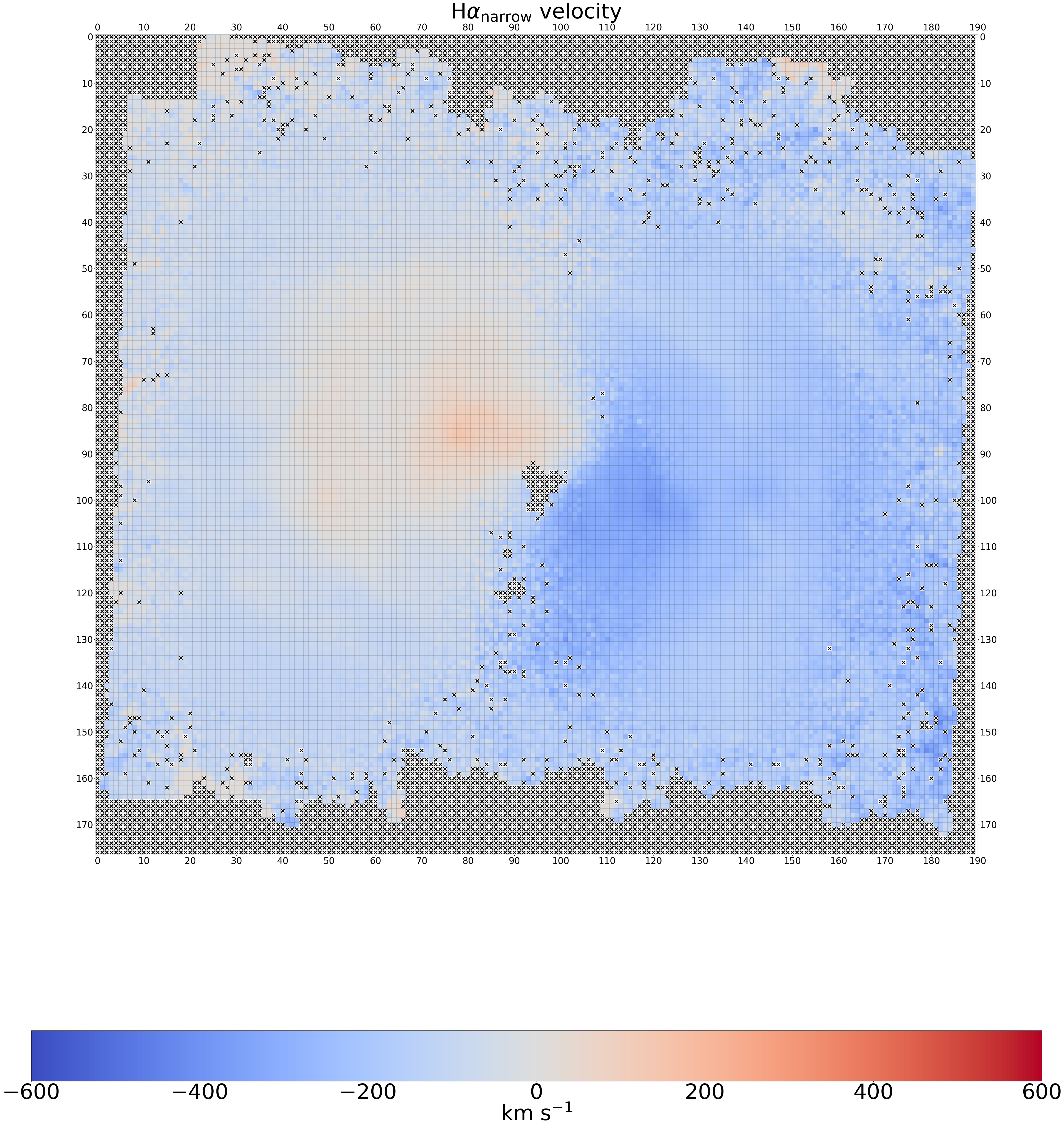
# Repeat steps **Select Valid Results** and **Fill Missing Point**
for _ in tqdm(range(500), desc="Processing"):
# Fill NaNs using the defined function
image_selected_fill_nan = fill_nan_with_median(image_selected)
upper_bound = image_selected_fill_nan + f1* sigma
lower_bound = image_selected_fill_nan - f1* sigma
for idx, image in enumerate(image_velocity_list):
# Iterate through all image sources
for i in range(image_selected.shape[0]):
for j in range(image_selected.shape[1]):
conditions_met = (
lower_bound[i, j] <= image[i, j] <= upper_bound[i, j] and
sigma_list[idx][i, j] <= f2 * sigma0 and
chi2_list[idx][i, j] < 1000
)
# If the selected image has NaN at this point, try to find a valid replacement
if np.isnan(image_selected[i, j]):
if conditions_met:
image_selected[i, j] = image[i, j] # Assign the value and stop searching
# If not NaN, check if a smoother value can be found
else:
if conditions_met: # A valid value is found
# If the current image is valid, calculate gradient smoothness
current_grad = gradient_sum(image_selected, i, j)
temp_image = image_selected.copy()
temp_image[i, j] = image[i, j]
new_grad = gradient_sum(temp_image, i, j)
if new_grad < current_grad:
# Replace the value if the new one leads to smoother gradient
image_selected[i, j] = image[i, j]
plt.figure(figsize=(60,70),dpi=100)
plt.imshow( image_selected,vmin = -600, vmax= 600, cmap='coolwarm' )
for i in range(image_selected.shape[0]):
for j in range(image_selected.shape[1]):
if np.isnan(image_selected[i, j]):
plt.plot([j-0.3, j+0.3], [i-0.3, i+0.3], 'k-', linewidth=3)
plt.plot([j+0.3, j-0.3], [i-0.3, i+0.3], 'k-', linewidth=3) # Draw a cross to mark NaN points
rect = plt.Rectangle((j-0.5, i-0.5), 1, 1, linewidth=0.1, edgecolor='black', facecolor='none')
plt.gca().add_patch(rect)
y_ticks = np.arange(0, (imax - imin) + 1, 10)
plt.yticks(y_ticks)
x_ticks = np.arange(0, (jmax - jmin) + 1, 10)
plt.xticks(x_ticks)
plt.tick_params(axis='both', which='major', labelsize=30)
plt.tick_params(axis='both', which='both', bottom=True, top=True, left=True, right=True, labelbottom=True, labeltop=True, labelleft=True, labelright=True)
plt.title(r'H$\alpha_{\rm narrow}$ velocity ',fontsize=70)
clb=plt.colorbar(orientation='horizontal')
clb.ax.tick_params(labelsize=70)
clb.ax.set_xlabel(r'km s$^{-1}$',fontsize=70)
plt.show()
sigma: 65.29440688552252
Processing: 100%|██████████| 500/500 [27:40<00:00, 3.32s/it]
[ ]:
# Get data folders
folder_names = []
for source in image_data_sources:
    # Get the variable name, preferably one starting with 'ha_vel'
    matching_names = [name for name, value in globals().items() if value is source]
    var_name = next(name for name in matching_names if name.startswith('ha_vel'))

    # Generate folder name based on the variable name
    if var_name == 'ha_vel':
        folder_name = 'reduced2'
    else:
        print(var_name)
        # Extract suffix from names like 'ha_vel_i83_93'
        suffix = var_name[len('ha_vel_'):]
        folder_name = f'reduced2_{suffix}'

    folder_names.append(folder_name)

# Generate folders dictionary
folders = {
    folder: f"ha_vel_{folder[len('reduced2')+1:]}" if folder.startswith('reduced2_') else 'ha_vel'
    for folder in folder_names
}
folders
[ ]:
# Copy files to the target folder
import os
import shutil

# Save the final selected fitting results to destination_folder

# Define the path to the destination folder
destination_folder = './reduced2_selected/'

# If the destination folder exists, delete it along with its contents
if os.path.exists(destination_folder):
    shutil.rmtree(destination_folder)

# Recreate an empty destination folder
os.makedirs(destination_folder)

# Iterate over image_selected to find non-NaN points,
# and copy the corresponding files from the selected source folder to the new folder
for i in range(image_selected.shape[0]):
    for j in range(image_selected.shape[1]):
        if not np.isnan(image_selected[i, j]):   # If this point is not NaN, it was selected

            # Loop through each image data source to find which one contributed the selected value
            for idx, (source_folder, vel_name) in enumerate(folders.items()):
                if np.isclose(image_selected[i, j], image_velocity_list[idx][i, j]):

                    file_name_fits = f'{i}_{j}.fits'
                    file_name_pdf = f'{i}_{j}.pdf'


                    # Source file paths
                    source_path_fits = os.path.join(source_folder, file_name_fits)
                    source_path_pdf = os.path.join(source_folder, file_name_pdf)

                    # Destination file paths
                    destination_path_fits = os.path.join(destination_folder, file_name_fits)
                    destination_path_pdf = os.path.join(destination_folder, file_name_pdf)

                    # Try copying the .fits file
                    try:
                        shutil.copy(source_path_fits, destination_path_fits)

                        # print(f"Successfully copied {file_name_fits} from {vel_name}!")
                    except FileNotFoundError:
                        print(f"文件 {file_name_fits} 在 {vel_name} 中未找到,跳过该文件。")

                    # Try copying the .pdf file
                    try:
                        shutil.copy(source_path_pdf, destination_path_pdf)
                        # print(f"Successfully copied {file_name_pdf} from {vel_name}!")
                    except FileNotFoundError:
                        print(f"文件 {file_name_pdf} 在 {vel_name} 中未找到,跳过该文件。")

                    # Once the matching file is found and copied, stop searching
                    break
plot the result(optional)
[ ]:
import numpy as np
import matplotlib.pyplot as plt
from matplotlib.colors import LogNorm
hasnr = np.load('./hasnr_selected.npy')
def plot_velocity_map(data, title=r'H$\alpha_{\rm na}$ velocity',
                     imin=0, imax=a, jmin=0, jmax=b,
                     vmin=-600, vmax=600):
    """
    Plot velocity map

    Parameters:
    -----------
    data : array-like
        Data to plot
    title : str, optional
        Title of the plot
    imin, imax : int, optional
        Row index range
    jmin, jmax : int, optional
        Column index range
    vmin, vmax : float, optional
        Minimum and maximum values for the color scale
    """

    data[hasnr < 5] = np.nan


    plt.figure(figsize=(60,70), dpi=100)
    plt.imshow(data[imin:imax, jmin:jmax], vmin=vmin, vmax=vmax, cmap='coolwarm',aspect='equal',origin='lower' )


    tick_labels = np.array([-4, -2, 0, 2, 4])
    x_ticks = (tick_labels / (- 7.03888888888889E-06*3600*2)) +190/2 - jmin
    plt.xticks(x_ticks, tick_labels)

    y_ticks = (tick_labels / (7.03888888888889E-06*3600*2)) +177/2 - imin
    plt.yticks(y_ticks, tick_labels)
    plt.tick_params(
        axis='both',
        which='both',
        labelsize=120,
        bottom=True,
        top=True,
        left=True,
        right=True,
        labelbottom=True,
        labeltop=False,
        labelleft=True,
        labelright=False,
         direction='in', length=40, width=10,pad=30
    )
    plt.xlabel(r"$\Delta  $RA[arcsec]", fontsize=120, labelpad=20)
    plt.ylabel(r"$\Delta $DEC[arcsec]", fontsize=120, labelpad=20)

    ax = plt.gca()
    for spine in ax.spines.values():
        spine.set_linewidth(10)


    plt.title(title, fontsize=150,pad = 100)
    clb = plt.colorbar(fraction=0.04, pad=0.04)


    clb.ax.tick_params(labelsize=100)


    clb.ax.yaxis.set_label_position('right')  # 将标题移到右侧
    clb.ax.set_ylabel(r'km s$^{-1}$', fontsize=140, labelpad=20)  # 设置标题和右边的距离

    # plt.savefig("i83_93.png",dpi =100)


    plt.show()
def plot_flux_map(data, title=r'H$\alpha_{\rm na}$ flux',
                  imin=0, imax=a, jmin=0, jmax=b,
                  vmin=1, vmax=100000):
    """
    Plot flux map

    Parameters:
    -----------
    data : array-like
        Flux data to plot
    title : str, optional
        Title of the plot
    imin, imax : int, optional
        Row index range
    jmin, jmax : int, optional
        Column index range
    vmin, vmax : float, optional
        Minimum and maximum values for the color scale
    """
    data[hasnr < 5] = np.nan

    plt.imshow(data[imin:imax, jmin:jmax], norm=LogNorm(vmin=vmin, vmax=vmax), cmap='inferno' ,aspect='equal',origin='lower' )


    tick_labels = np.array([-4, -2, 0, 2, 4])
    x_ticks = (tick_labels / (- 7.03888888888889E-06*3600*2)) +190/2 - jmin
    plt.xticks(x_ticks, tick_labels)

    y_ticks = (tick_labels / (7.03888888888889E-06*3600*2)) +177/2 - imin
    plt.yticks(y_ticks, tick_labels)
    plt.tick_params(
        axis='both',
        which='both',
        labelsize=120,
        bottom=True,
        top=True,
        left=True,
        right=True,
        labelbottom=True,
        labeltop=False,
        labelleft=True,
        labelright=False,
         direction='in', length=40, width=10,pad=30
    )
    plt.xlabel(r"$\Delta  $RA[arcsec]", fontsize=120, labelpad=20)
    plt.ylabel(r"$\Delta $DEC[arcsec]", fontsize=120, labelpad=20)

    ax = plt.gca()
    for spine in ax.spines.values():
        spine.set_linewidth(10)


    plt.title(title, fontsize=150,pad = 100)

    clb = plt.colorbar(fraction=0.04, pad=0.04)

    clb.ax.tick_params(labelsize=100)


    clb.ax.yaxis.set_label_position('right')  # 将标题移到右侧
    clb.ax.set_ylabel(r'$\rm 10^{-20}\ erg\ s^{-1}\ cm^{-2}$', fontsize=140, labelpad=20)  # 设置标题和右边的距离

    # plt.savefig("16.png",dpi =100)


    plt.show()


# plot_velocity_map((np.e**ha_vel_i83_93-6564.4)/6564.4*3e5,vmin=-350,vmax=350, title=r'H$\alpha_{\rm na}$ velocity')

# plot_velocity_map((np.e**ha_vel_median-6564.4)/6564.4*3e5,vmin=-300,vmax=300, title=r'H$\alpha_{\rm narrow}$ velocity(median refitted)')


var_name = "ha_vel_selected"

plot_velocity_map((np.e**(globals()[var_name]) - 6564.4) / 6564.4 * 3e5,vmin=-350,vmax=350, title=r'H$\alpha_{\rm narrow}$ velocity (optimized)')


A = globals()['ha_flux_flat']
mu = globals()['ha_vel_flat']
c = globals()['ha_sigma_flat']
area = np.sqrt(2 * np.pi)*A * c*np.exp(mu + (c**2) / 2)
plot_flux_map(area,title=r'H$\alpha_{\rm na}$ flux')


# plot_flux_map(ha_flux_j109_119, title=r'H$\alpha_{\rm narrow}$ flux (j109_119)')