Select the Best Fitting Results
After following the procedure in Quick Start Guide, each spectrum of the IFS data will have a fitting result. By changing the function parameters, different fitting results can be obtained. In this section, we provide a method for selecting different fitting results. The general workflow is as follows.
Define Selection Region
In the initial velocity map of the \(\text{H}\alpha\) narrow component, the user selects regions where the fitting results are relatively smooth and physically plausible. After removing points with sudden velocity changes, these selected points are used as the initial reference. Here is a schematic illustration of the selected regions.
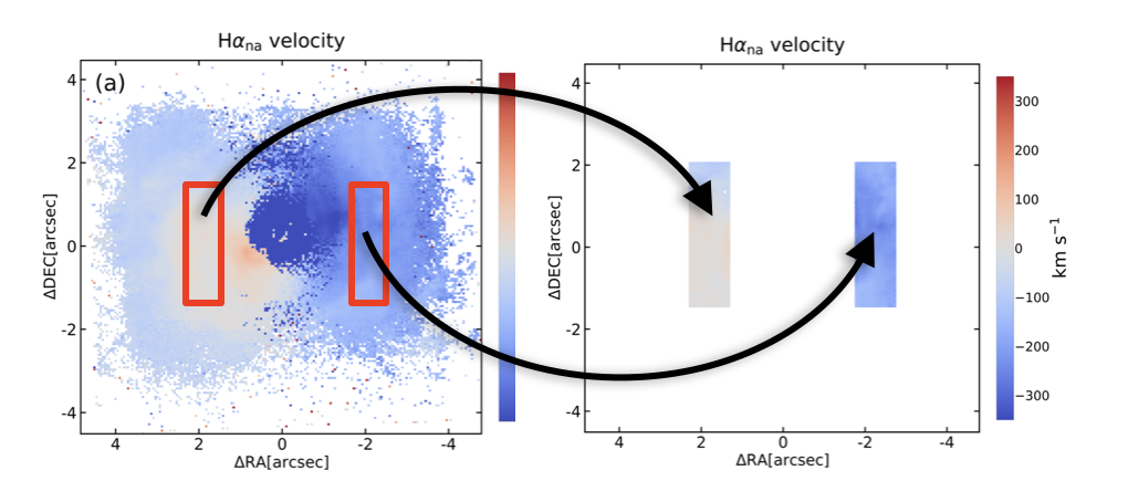
Schematic illustration of the selected regions
The median of the velocity broadening of the \(\text{H}\alpha\) narrow
component in these points is taken as sigma0.
Select Valid Results
For each set of emission line fitting results, if the difference between the velocity of the \(\text{H}\alpha\) narrow component and the
initial velocity map is within the range of f1*sigma0, and the velocity broadening of the \(\text{H}\alpha\) narrow component is
less than f2*sigma0, it is selected; otherwise, it is excluded. Here, f1 and f2 are user-defined parameters. Recommended thresholds are f1 < 3 and f2 < 5 (e.g., f1 = 1.5, f2 = 2).If multiple results
are selected for a single pixel, the one with the smallest sum of absolute differences from the surrounding results, i.e., the one with the
most continuous fitting, is automatically chosen.
Fill Missing Point
After obtaining the first round of selected results, these results are used as the basis for further selection. For points that are not selected, if more than three surrounding points are selected, the median of the surrounding velocity values is taken as the basis for selection.
Repeat
Repeat steps Select Valid Results and Fill Missing Point until the set number of iterations is reached. In this way, the result obtained for each pixel is considered spatially continuous.

Selection flowchart
As before, we continue to use MR 2251−178 as an example. The following panels show the results obtained from different fitting strategies, along with the selected results based on the methods described above. It can be seen that the fitting results are not only smoother above and below the target source, but also significantly improved in the central region near the source.
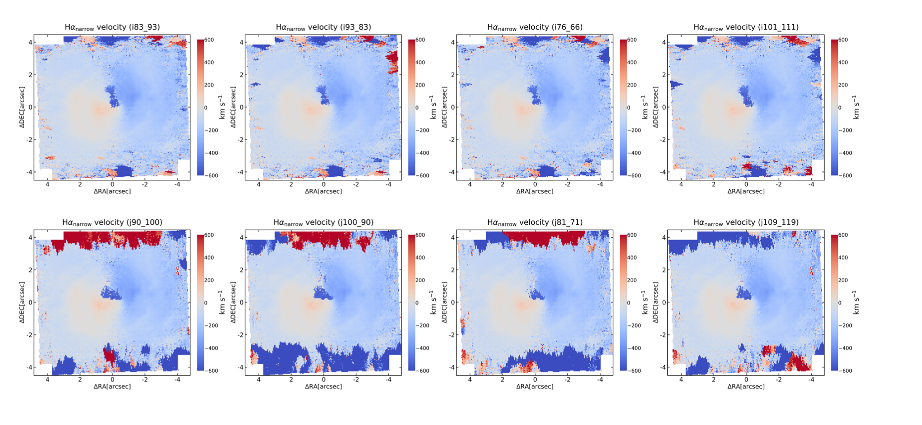
Results obtained from different fitting schemes
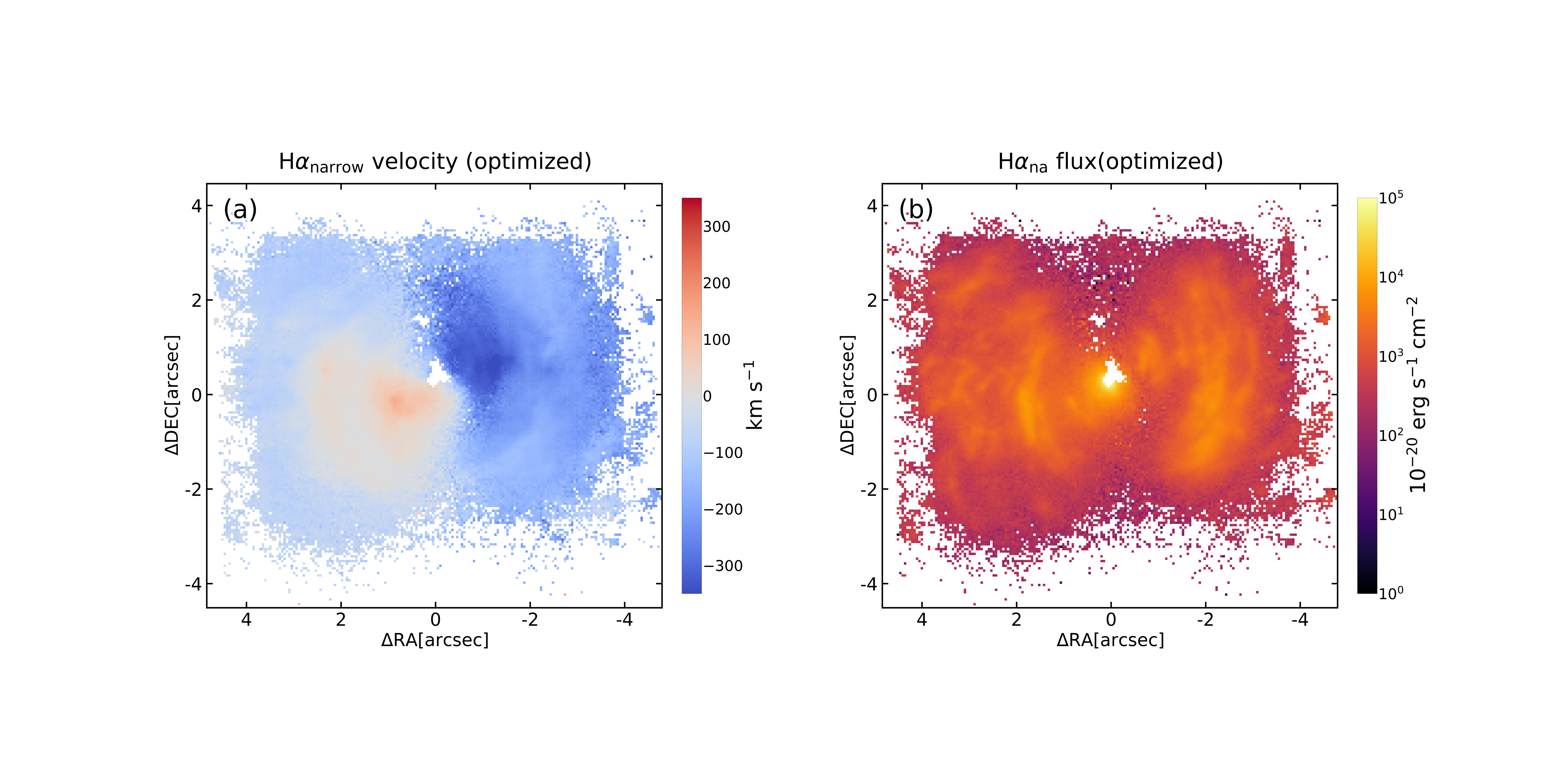
The results selected using the above procedure
Code
The Jupyter notebook used to select the fitting results in this example is provided here for reference.