Quick Start Guide
Installation
csst-ifs-elfo can be installed as follows:
1git clone https://csst-tb.bao.ac.cn/code/csst-pipeline/ifs/csst_ifs_elfo.git
2cd csst-ifs-elfo
3python -m pip install .
Prepare the IFS data
The IFS simulated observation data from CSST can be downloaded from the following link: Download.
Import Required Modules and Functions
Import the functions from csst-ifs-elfo to perform the fitting:
from elfo import process_i_refit
from elfo import process_j_refit
Note
Both functions share the same fitting logic, fitting the spectra column by column.
The only difference lies in the direction of progression process_i_refit proceeds along rows,
while process_j_refit proceeds along columns.
The fitting of the IFS data is performed using the two imported functions.
In the following, we take process_i_refit as an example, which fits all spectra using the fitting results of adjacent rows.
For a detailed description of the fitting strategy, see the ELFO workflow section below, where we explain how ELFO’s process_i_refit
function specifically fits the IFS data.
Parameters
i_1: The starting row index for the first fitting. Type:int.i_2: The starting row index for the second fitting. Type:int.fits_file: The path to the input FITS file. Type:str.z: Redshift of the target object. Type:float.scale_factor(optional): The scale factor for rebinning the IFU spectra. Default is1. Type:int.flux_cube_path(optional): The file path to the flux cube of the IFU data. (for pre-binned spectra)Default isNone. Type:str.var_cube_path(optional): The file path to the variance cube of the IFU data. (for pre-binned spectra)Default isNone. Type:str.format(optional): The format of the input FITS file. Default is'muse'. Type:str.
Returns
str: The path to the output directory where the results are saved.
Set up the model input parameters
See an example in the example notbook.
Run the Fitting
Usage Example
Once the IFS data is ready and the functions are imported, we can run the fitting.
1path_out = process_i_refit(i_1=30, i_2=20, fits_file='CSST_IFS_CUBE.fits', z=0.003373, format='csst')
2# Using optional parameters for custom flux/var cubes and scale factor (for pre-binned spectra)
3path_out = process_i_refit(i_1=80, i_1=90, fits_file='example.fits', z=0.02, scale_factor=2, flux_cube_path='reduced2_flux.npy', var_cube_path='reduced2_var.npy', format='csst')
The function will automatically save the fitting results to the returned path (path_out).
For each spectrum, PyQSOFit generates a .fits file with parameters and a .pdf showing the fitting result.
More details on the fitting process can be found in the ELFO workflow section below.
Here is an example using MUSE spectral fitting of the quasar MR 2251−178 to demonstrate the improvement brought by ELFO in emission-line fitting. The upper panel shows the velocity and flux maps of the \(\text{H}\alpha\) narrow component obtained by fitting each spectrum individually using the default initial parameters in PyQSOFit. In contrast, ELFO utilizes the best-fitting result from neighboring points as the initial guess for each fit.
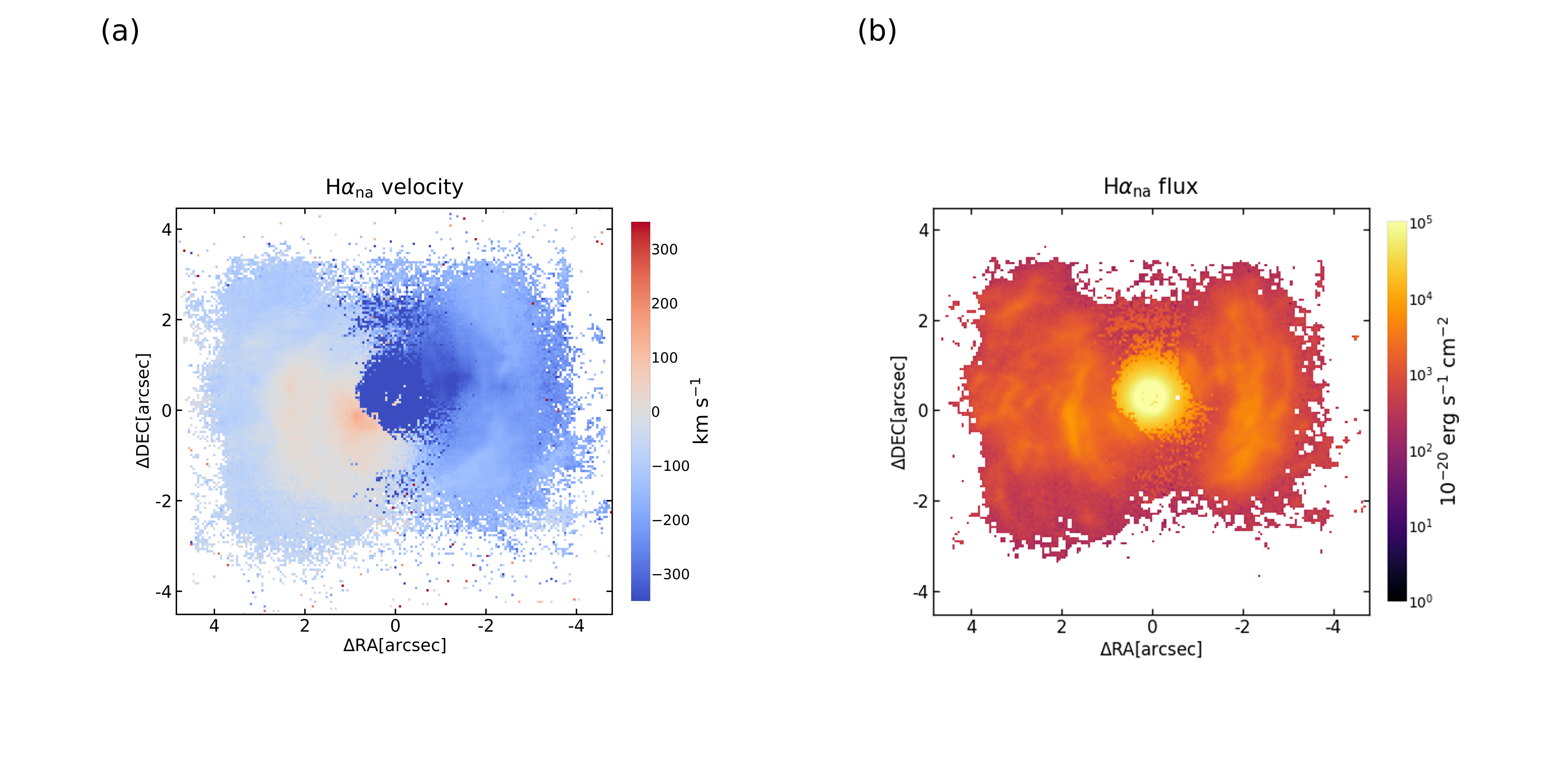
The result obtained by fitting each spectrum with the default parameters
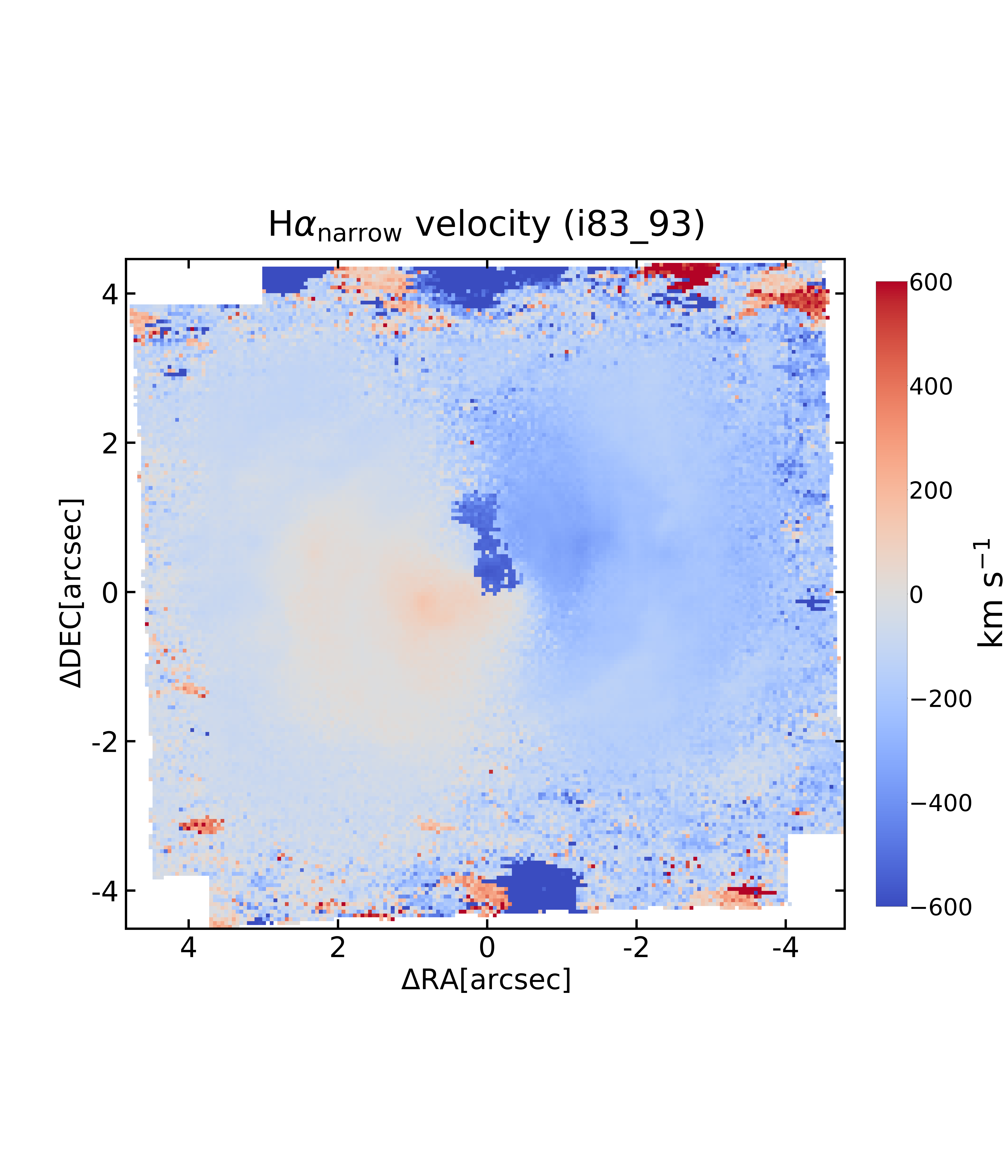
The result obtained by using the best fit from neighboring points as the initial guess for each spectrum.